Understanding protein inference

Bottom-up and middle-down experiments begin by digesting proteins into peptides. These are run through LC-MS/MS, producing a raw file containing MS/MS spectra. Mascot does the same in silico: a protein sequence database is digested into peptide sequences and these are matched to the MS/MS spectra.

The next, key step for protein identification is protein inference. The software must deduce which proteins were in the sample based on the identified peptides. Mascot’s protein inference is a novel algorithm that uses information from both unique and shared peptides to build a complete picture.

Motivation

The goal of a shotgun proteomics experiment is not the creation of a table of proteins for a publication; it is to gain insight into a biological system.

The goal of a summary report is to present a minimal list of the possible protein assignments clearly, so that someone with knowledge of the biology can make an informed decision as to which proteins are present. The summary report must facilitate answering questions such as:

• For which proteins do we need to make antibodies?
• Is there evidence for a particular isoform of this protein?
• Does this protein carry a biologically interesting modification or polymorphism?
• Which proteins have been up- or down-regulated?

If you get a good match to a peptide sequence that is unique to a protein, obviously the protein has to be present in the sample. However, in most cases, the matched peptides will not be unique to a single protein, and there will be some ambiguity about precisely which proteins are present.

Real-life data sets searched against public protein sequence databases present certain complications. Due to natural variants, the sequence of a particular protein in the database will often differ from the sequence of the protein in the sample. If we get matches to two similar sequences, the truth may be that the analyte is partly represented by one database entry and partly represented by the other. In such cases, it is misleading to report that only one is present or that both are present.

On the other hand, consider a non-identical database containing two homologous protein sequences, maybe 90% identical. Whether we get peptide matches to one or both, a protein inference algorithm that excludes shared peptide matches would mean that neither protein appears in the result report, which is actively misleading.

You can mask inference problems by selecting a highly non-redundant database, which collapses similar proteins into a single, canonical sequence. This may be fine for a rough survey, but the drawback is that some PSMs are lost because the target peptide sequence didn’t make it into a canonical sequence. For a well characterised organism, the most sensitive and accurate search results come from searching a database such as a UniProt proteome with isoforms.

Five categories of protein similarity

The diagram below illustrates the five categories of protein similarity. The shaded regions are peptide matches.

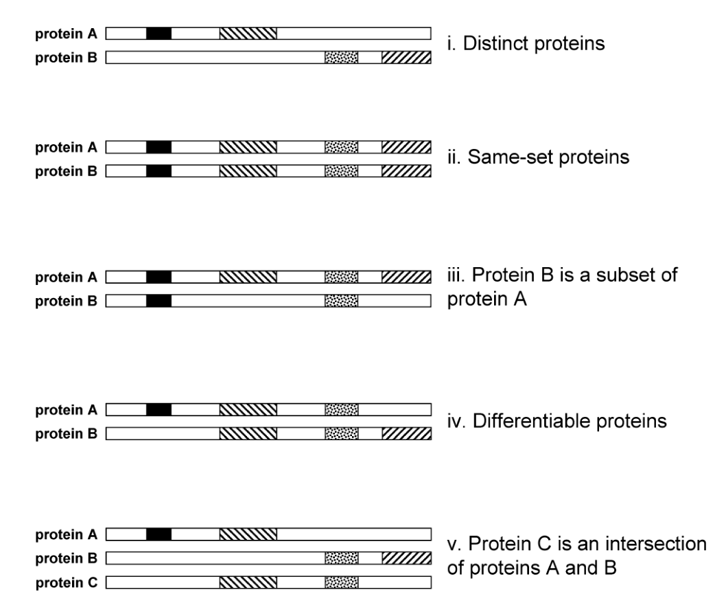
Two proteins are distinct when they share no peptide matches. Two proteins are differentiable when they share some peptide matches but each have unique evidence. In both cases, a summary report should list these at a top level.

There can be complete ambiguity when two proteins have identical peptide matches. These sameset proteins are indistinguishable based on the MS/MS evidence alone.

Cases with more complex ambiguity are intersections, where all peptide matches of a protein are explained by other proteins. A special case is subset protein, which is entirely subsumed in another protein.

Protein Family Summary

Mascot solves protein inference by grouping proteins into ‘families’ based on shared peptide matches. Then, proteins within a family are hierarchically clustered based on unique peptides. The end result is:

• All protein hits reported as top-level family members have unique, statistically significant peptide evidence. These are the differentiable proteins.
• Homologous proteins and isoforms are grouped together.
• Any two families are distinct, because they share no peptide matches.
• Sameset proteins are collated into a single representative protein. Because there is no MS/MS evidence to disambiguate, the representative is chosen arbitrarily: numerically or alphabetically first protein accession. (This can be controlled by selecting a preferred taxonomy.)
• Proteins with no unique peptide evidence are collated into subsets/intersections. These proteins are not necessarily absent from the sample; there is simply no direct evidence for them.
• Only statistically significant peptide matches are used for protein inference. (That is, the peptide match score must exceed the score threshold at the target FDR.)

If it is essential to characterise the complete protein sequence, or to choose between splice variants, or to confirm a SNP, it is likely that additional, targeted experiments will be required.

Previous versions of Mascot Server

Protein Family Summary was introduced in Mascot Server 2.3. An older protein grouping algorithm is used by legacy summary reports. These reports are still available, but they will be removed in a future Mascot release.

Example

This example is from a benchmarking data set published in The et al., J Prot Res, 17(5), 2018. Briefly, a collection of human Protein Epitope Signature Tags (PrESTs) were expressed in E. coli and 191 overlapping pairs selected so that each pair would have some unique and some shared tryptic peptides. The pairs were divided into two pools, A and B, and a third pool was created by combining A and B.

The data were peak picked with Mascot Distiller and searched against the combined E. coli and human UniProt proteomes, including isoforms. The screenshot below illustrates a small protein family from the A+B pool.

The key elements of protein inference are apparent. Q8N0S6, Q8N0S6-2 and Q8N0S6-3 are isoforms of CENPL_HUMAN. They share a number of peptide matches, so Mascot groups them into the same protein family. Because Q8N0S6 and Q8N0S6-2 both have unique peptide matches, they are presented as family members and separated by hierarchical clustering. Isoform 3 becomes an intersection protein, because all of the peptide matches can be accounted for by the other two isoforms.

The unique peptides are R.DPEAFLVQIVSK.S and K.GTQRDPEAFLVQIVSK.S. These are only found in isoform 1 while K.GTQRDPEAFLVQGLILSPR.L is only found in isoforms 2 and 3. The scores of the best matches to these peptides – 88, 70, 79 respectively – are used for the distance metric in the dendrogram for Q8N0S6 and Q8N0S6-2.

It is worth noting that the unique peptide sequences (marked ‘U’) are unique to this protein family in the whole database search. If they were shared with any other protein, those proteins would have been grouped into the same family.

If we searched only the canonical sequences, we would not see the matches to K.GTQRDPEAFLVQGLILSPR.L and it would be easy to assume we had a single protein. If we searched the complete database but excluded shared PSMs, we would discard the evidence that favours isoform 2 over isoform 3. Also, if a two-peptide rule was applied, we would only report a single protein, which again, is incorrect. We have ground truth for this sample, and the peptides map to two different splice variants.

The Algorithm

The full Protein Family Summary algorithm is described in Koskinen, V. R., Hierarchical Clustering of Shotgun Proteomics Data 2011 MCP 10 M110.003822. Below is an overview of the steps.

Grouping proteins

The database search results consist of peptide-spectrum matches. Each peptide match has a list of the protein accessions where the peptide sequence is found. Mascot initially collates the protein hits in a simple way, so that a protein hit contains a list of all of its peptide matches. The protein is given a score calculated from the peptide matches.

The grouping algorithm begins from the list of protein hits:

1. Sort the list by protein score.
2. Take the highest scoring protein hit.
3. Find all the family members for this protein by looping the below steps:
   • select all statistically significant peptide matches assigned to the protein hit
   • for each peptide match, select all other the proteins that match the same peptide sequence, ignoring modifications and charge state (peptide matches with I to L substitution or other differences that have no impact on the score are treated as the same sequence)
   • for each new protein, select all of its statistically significant peptide matches and add them to the queue
   • loop until all related proteins and peptide matches have been found
4. Report this family as a single unit. All these proteins can be removed from the list.
5. For each protein in the family, make a list of the distinct peptide sequences. That is, ignore differences in score, modifications, charge, etc. Duplicate matches to the same sequence are collated into the highest scoring match.
6. Divide and group the proteins into sameset proteins and intersection proteins (including subset proteins):
   • where there are sameset proteins, collapse into a single family member and choose a representative protein
   • move any proteins that are subsets or intersections to the subsets list
7. Perform hierarchical clustering on the family members (see below), using the score excess over threshold of the unique peptides as the distance metric.
8. Loop from step 2 until no more proteins remain that contain significant peptide matches.

Note that, if you select a pair of family members from a large family, it is perfectly possible that they will have no shared matches. Each family member will have shared matches with at least one other family member, or they would not have been grouped into the same family, but this doesn’t mean that there are going to be shared matches between every pair.

Hierarchical clustering within a family

The hierarchical clustering algorithm that separates family members uses a distance metric based on unique peptide matches:

1. If two proteins have the same set of peptide matches, the distance between them is zero.
2. Otherwise, the distance is the sum of the score excesses of all the unique peptide matches in one protein. This metric is asymmetric, and the score distance to make protein A into a subset of protein B will not be the same as that to make B a subset of A. The smaller distance is always chosen.

Corner cases

There are some subtleties to the hierarchical clustering. Consider the case of two proteins which have different peptide matches to the same query with the same score. Only one of these matches can be correct, but we don’t know which.

One obvious example is where the two sequences differ only in exchange of I and L. In terms of the mass spectrum, these sequences are identical. Unless the mass accuracy is high, the same is true for exchange of Q and K or F and oxidised M. Clearly, a sequence containing F at a particular position is very different, in biological terms, from one containing M at the same position. But, if the scores are the same, there is simply no evidence from the mass spectrometry data for two proteins. In terms of a distance matrix, we must treat it is as if there was no match to either peptide.

Now, consider the case where we have two proteins with different peptide matches to the same query and the scores are not the same. Assume the threshold is 40 and one has a score of 50 and the other has a score of 60. Again, only one of these matches can be correct; it is not the same as if they were independent matches to different queries. Extending the logic that matches to the same query with the same score correspond to a distance of zero, matches to the same query with different scores correspond to a distance that is the score difference. In this example, the distance would be 10. If the two matches came from different queries, and could be treated independently, the distance would be (60 – 40) + (50 – 40) = 30.

Creating the dendrogram

To create the dendrogram, we first compute a distance matrix, which is the distance between each pair of proteins. The two proteins separated by the smallest distance are joined to create a node, with the length of the branches from the node are the score distance between the proteins. The two joined proteins are removed from list, replaced by the node, and the distances between the new node and all other remaining proteins (or nodes) computed. The process is repeated until only one node remains.

When the dendrogram (or tree) is drawn, the order is chosen to avoid any branches crossing. There is no other significance to the order of the branches, and there are many possible ways to order the branches so as to avoid crossings. In the tabular part of the report, proteins are sorted in order of decreasing score, and this will often be different from the dendrogram order.